Transformer Architecture

A transformer is a neural network architecture proposed in Google’s 2017 paper Attention is All You Need. It is the basis of many NLP models such as BERT, GPT, etc. This article seeks to describe the transformer from the background to the details of the model.

Self-Attention

Consider a key-value database that returns the value after finding the desired data through the key when a user enters a query through the search bar.

Key (Title)	Value (URL)
My dog is happy!	www.youtube.com/my_dog_is_happy
VLOG in Zürich	www.youtube.com/VLOG_in_zurich
…	…

If a query “dog videos” is given from a user, it would be appropriate to provide the video corresponding to the first key to the user because the first key “My dog is happy!” is more similar to the query than the second key “VLOG in Zürich”.

Self-attention was inspired by the retrieval system of the database. The three mentioned above (query, key, value) are components of self-attention.

• Query \(\mathbf Q\)
• Key \(\mathbf K\)
• Value \(\mathbf V\)

Self-attention is a way to find the relationship between each token \(x_i\) in the sequential data \(\mathbf x = (x_1, \dots, x_n)\). The code below is a simple implementation of self-attention.

score = [[0] * n for _ in range(n)]

for i in range(n):
	# for a query x_i
	for j in range(n):
		# for a key x_j
    	score[i][j] = score(x[i], x[j])

When \(x_i\) is query and \(x_j\) is key, we find out how related they are through the function \(\operatorname{score}(x_i, x_j)\).

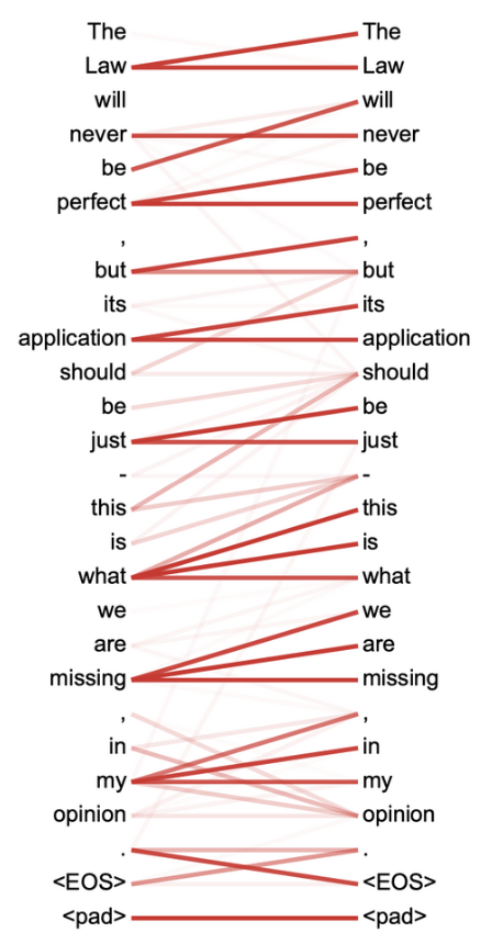
The figure above illustrates the \(\operatorname{score}(x_i, x_j)\) of the trained transformer. When the token on the left is given as a query, we can see that the token with a high relevance has a high \(\operatorname{score}(x_i, x_j)\).

Then, how do we calculate \(q_i\) and \(k_j\)? In the transformer, we use the transformation matrix \(W^Q\) and \(W^K\) to get \(q_i\) and \(k_i\) from \(x_i\).

\[\begin{aligned} q_i &= x_i W^Q \\ k_j &= x_j W^K \end{aligned}\]

Here, the inner product \(q_i \cdot k_j\) of \(q_i\) and \(k_j\) is \(\operatorname{score}(x_i, x_j)\).

Therefore,

\[\operatorname{score}(x_i, x_j) = q_i \cdot k_j = q_i k_j^\intercal,\]

and if we combine all queries \(q_1, \dots, q_n\) into a matrix \(Q = (q_1, \dots, q_n)\) and all keys \(k_1, \cdots,k_n\) into \(K = (k_1, \dots, k_n)\), then

\[\begin{aligned} \operatorname{score}(x_i, x_j) &= row_i(Q) \cdot row_j(K) \\ &= row_i (Q) column_j(K^\intercal) \\ &= (QK^\intercal)_{ij} \end{aligned}.\]

Here, \(QK^\intercal\) is the relevance when \(x_i\) is query and \(x_j\) is key. In other words, \(QK^\intercal\) calculated from \(\mathbf x\) means the relevance between \(x_i\) as query and \(x_j\) as key.

However, if the dimensionality \(d_k\) of the embedding space where the token exists is large, \(QK^\intercal\) can become infinitely large as \(d_k\) increases, which can cause problems during computer operations. Therefore, we divide it by \(\sqrt{d_k}\).

\[QK^\intercal \rightarrow \frac{QK^\intercal}{\sqrt{d_k}}\]

To interpret “how relevant each key \(k_j\) is when query \(q_i\) is given”, it would be more reasonable to normalize the value by \(\operatorname{softmax}\) than to use the value as it is.

\[QK^\intercal \rightarrow \frac{QK^\intercal}{\sqrt{d_k}} \rightarrow \operatorname{softmax}(\frac{QK^\intercal}{\sqrt{d_k}})\]

translate: It may be a little strange to take \(\operatorname{softmax}\) on a matrix, but as explained above, it is correct to normalize the relevance between query \(q_i\) and key \(k_j\) when a certain query \(q_i\) is given, so take \(\operatorname{softmax}\) on the row of the matrix \(\operatorname{softmax}(\frac{QK^\intercal}{\sqrt{d_k}})\).

Finally, multiply the value \(V = (v_1, \dots, v_n)\) to the normalized matrix. \(v_i\) is also obtained by multiplying \(v_i = x_i W^V\), so

\[\operatorname{SelfAttention}(\mathbf x) = \operatorname{softmax}(\frac{QK^\intercal}{\sqrt{d_k}})V.\]

This is the self-attention of the transformer. In the paper Attention is All You Need, this is called Scaled Dot-Product Attention.

Multi-Head Attention

As mentioned above, self-attention is a way to find the relationship between each token \(x_i\) in the sequential data \(\mathbf x = (x_1, \dots, x_n)\). However, some sequential data are not connected by one thing, but are connected by several factors. For example, in the case of text, there may be synonyms or parts of speech.

In order to capture these various relationships, multi-head attention uses \(\operatorname{SelfAttention}\) with different \((W^Q, W^K, W^V)\) for the same sequential data \(\mathbf x\). If indexed by \(i\),

\[\operatorname{SelfAttention}_i(\mathbf x) = \operatorname{softmax}(\frac{QK^\intercal}{\sqrt{d_k}})V.\]

Here, \(\operatorname{SelfAttention}_i\) is the \(i\)th \(\operatorname{SelfAttention}\), and there will be \(W_i^Q, W_i^K, W_i^V\) to obtain \((Q, K, V)\) corresponding to \(\operatorname{SelfAttention}_i\).

Multi-head attention concatenates the results obtained by using these several \(\operatorname{SelfAttention}_i\) as input \(\mathbf x\), that is, concatenates them, and then uses the operator \(W^O\) to project them to match the dimension of the input again. In multi-head attention, \(\operatorname{SelfAttention}_i\) is called \(\operatorname{head}_i\) instead, and in summary,

\[\operatorname{MultiHeadAttnention}(\mathbf x) = \operatorname{Concat}(\operatorname{head}_1(\mathbf x), \dots , \operatorname{head}_h(\mathbf x)) W^O.\]

Model Architecture

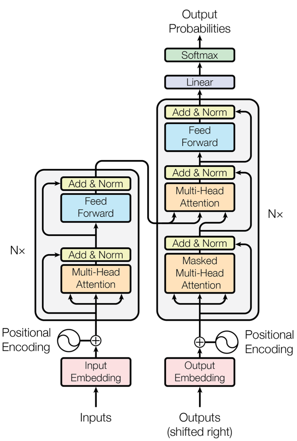
This is the basic architecture of the transformer. The left part is the encoder and the right part is the decoder. The \(N \times\) in the figure means that the structure is stacked \(N\) times, but the transformer block, which is called the transformer block, has a slightly different structure for the encoder and decoder. In the paper, both the encoder and the decoder were stacked 6 times. (\(N = 6\))

Transformer Block

1. Input \(\mathbf x\)

\(\mathbf x\) is the input.

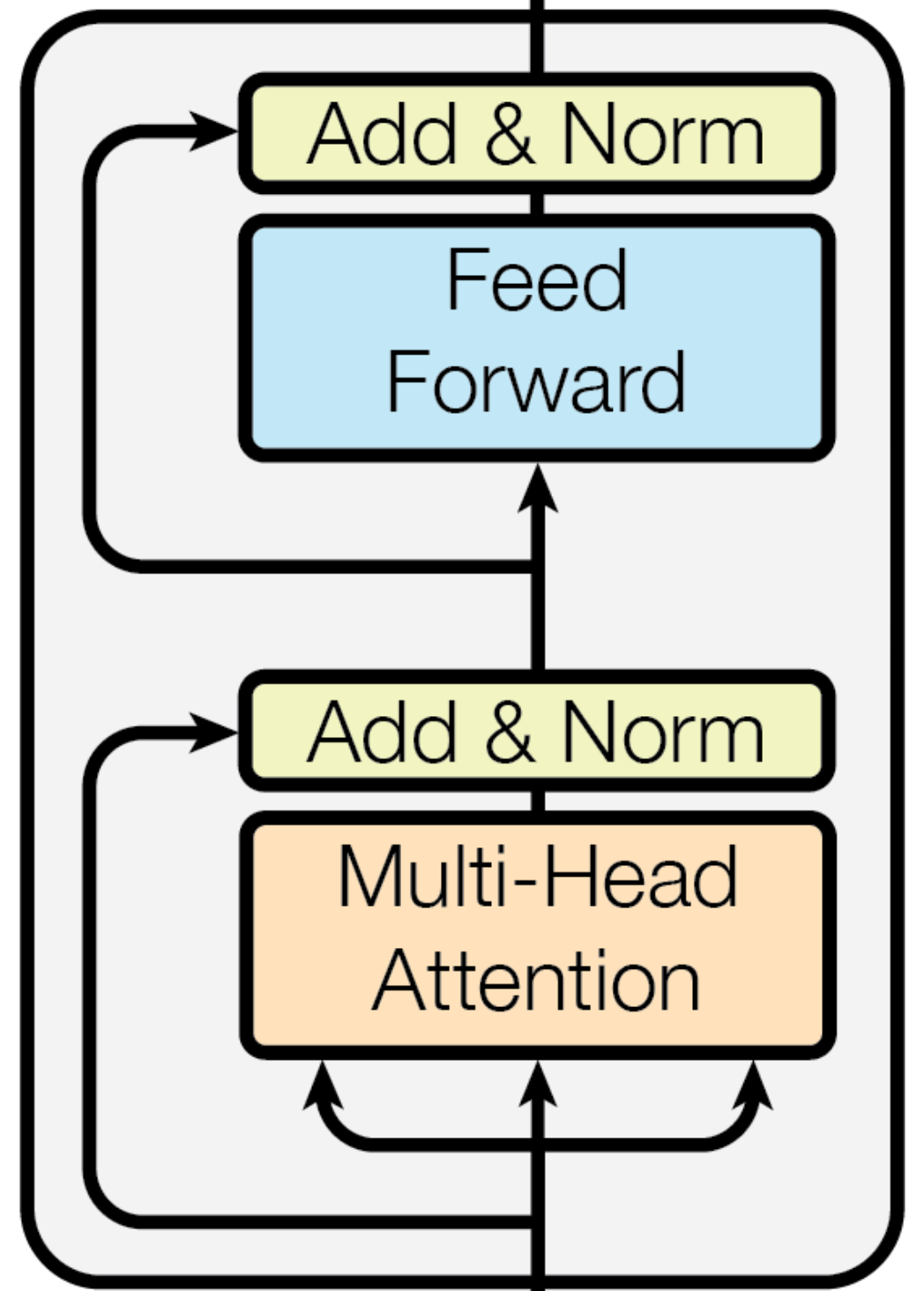
2. Multi-Head Attention, Add & Norm

For each input \(\mathbf x\), the operations are as follows:

1. Multi-head attention,
2. Residual connection,
3. Layer normalization.

Mathematically, it can be expressed as follows:

\[\mathbf z = \operatorname{LayerNorm}(\mathbf x + \operatorname{MultiHeadAttention}(\mathbf x))\]

Multi-Head Attention

The multi-head attention mechanism is formalized as:

\[\operatorname{MultiHeadAttnention}(\mathbf x) = \operatorname{Concat}(\operatorname{head}_1(\mathbf x), \dots , \operatorname{head}_h(\mathbf x)) \mathbf W^O\] \[\operatorname{head}_i (\mathbf x) = \operatorname{SelfAttention}(\mathbf Q, \mathbf K, \mathbf V) = \operatorname{softmax}\left(\frac{\mathbf Q \mathbf K^\intercal}{\sqrt{d_k}} \right) \mathbf V\]

where

• Query \(\mathbf Q = \mathbf x \mathbf W_i^Q\)
• Key \(\mathbf K = \mathbf x \mathbf W_i^K\)
• Value \(\mathbf V = \mathbf x \mathbf W_i^V\)
• Dimensionality \(d_k = dim(\mathbf V)\)

Residual Connection

The equation \(\mathbf x + \operatorname{MultiHeadAttention}(\mathbf x)\) encapsulates the residual connection, serving as a corrective term to mitigate issues arising from vanishing gradients during recurrent network training.

Layer Normalization

Layer normalization is expressed as:

\(\mathbf z = \operatorname{LayerNorm}(\mathbf x + \operatorname{MultiHeadAttention}(\mathbf x))\)**

\[\operatorname{LayerNorm}(\mathbf a) = \left( \frac{\mathbf a - \mathbb E[\mathbf a]}{\sqrt{\operatorname{Var}[\mathbf a] + \epsilon}} \right) * \gamma + \beta.\]

Here, \(\gamma\) and \(\beta\) are learnable parameters, representing gain and offset, respectively.

3. Feed Forward & Add & Norm

The final output sequence \(\mathbf y\) is obtained as: \(\mathbf y = \operatorname{LayerNorm}(\mathbf z + \operatorname{FFN}(\mathbf z))\)

4. Output \(\mathbf y\)

The output sequence, \(\mathbf y\), is the final product of the transformation block.